Scarica il documento per vederlo tutto.
Scarica il documento per vederlo tutto.
Scarica il documento per vederlo tutto.
Scarica il documento per vederlo tutto.
Scarica il documento per vederlo tutto.
Scarica il documento per vederlo tutto.
Scarica il documento per vederlo tutto.
Scarica il documento per vederlo tutto.
Scarica il documento per vederlo tutto.
Scarica il documento per vederlo tutto.
Scarica il documento per vederlo tutto.
Scarica il documento per vederlo tutto.
Scarica il documento per vederlo tutto.
Scarica il documento per vederlo tutto.
vuoi
o PayPal
tutte le volte che vuoi
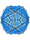 The goal of this work is to present a study of the natural vibrations of spherical viral capsids - we think, in particular, of the Satellite Tobacco Mosaic Virus (STMV) and of the Cowpea Chlorotic Mottle Virus (CCMV) - by employing a continuum mechanics approach. We model such capsids as linearly elastic shells, whose response at any point is transversely isotropic with respect to the radial direction through that point (the simplest and most important subcase, isotropic response, is almost invariably considered in literature). Our choice is motivated by the desire to account for the rotational symmetries with respect to the radial direction of capsomers, the functional units a capsid consists of. In addition to transverse isotropy, the shell theory we employ has some other unusual traits.
Francesco Bonaldi, A Continuum Theory for the Natural Vibrations of Spherical Viral Capsids, Tesi di laurea in Ingegneria matematica.
Z
s s β ⊗
F (x, t) := α(x, ζ)S(x, ζ; t) B(x, ζ) dζ = αSg dζ e ,
β
I I
Z
Z
s s β (4.2)
⊗
M (x, t) := α(x, ζ)ζS(x, ζ; t) B(x, ζ) dζ = αζSg dζ e ,
β
I I
Z
(3)
f (x, t) := α(x, ζ)S(x, ζ; t)n(x) dζ.
I (3)
s s
We call F the M the and f the
force tensor, moment tensor shear vector.
4.1.2 External Virtual Work
The system of external loads is made of: ni in
• the per unit volume d = d + d , the former addend
distance force o o o
being its part, the latter its part. Denoting the mass
non-inertial inertial
density of the shell by δ , we have
o
in −δ
d (x, ζ; t) = ü(x, ζ; t);
o
o
• the c per unit area, acting on the boundary ∂G of the shell.
contact force o 33
4.1. WEAK FORMULATION
− ±
+
S ∪S S {x ± ∈ S},
We write ∂G = , where := εn(x) : x and use the notation
± ±ε)
Ψ (x) := Ψ(x,
±
S
for the restriction of a field Ψ to .
The expenditure of over the shell-like body is
external virtual work
Z Z
ext
W · ·
(G) [δu] := d δu + c δu.
o o
G ∂G
Again, choosing δu of the same form as (3.1) and following the same procedure
set forth in [7], we get Z
ext
W {q · · · ·
(G) [δa, δw, δϕ, δγ] = δa + (q n)δw + r δϕ + (r n)δγ} ,
o o
o o
S (4.3)
where Z − −
+ +
q (x, t) := α(x, ζ) d (x, ζ; t) dζ + α (x)c (x) + α (x)c (x),
o
o o o
I
Z (4.4)
− −
+ + −
α(x, ζ)ζd (x, ζ; t) dζ + ε α (x)c (x) α (x)c (x)
r (x, t) := o
o o o
I
are the and the per unit area, respectively. The
distance force distance couple
in ni
decomposition d = d + d implies analogous decompositions for q and r :
o o
o
o o
in ni in ni
q = q + q , r = r + r ; in particular, we find that
o
o o o o o
Z
(1)
(0)
2 2 2 2
ε ∂ u 2ε ∂ u
in
in −2εδ
α(x, ζ) d (x, ζ; t) dζ = 1+ (x, t) + (x, t) ,
q (x, t) = o
o o
2 2 2
3ρ ∂t 3ρ ∂t
o
I o
Z
(0) (1)
2
2 2
2 ∂ u 1 ε ∂ u
in 3
in −2ε
α(x, ζ)ζd (x, ζ; t) dζ = δ
r (x, t) = (x, t) + + (x, t) .
o
o o
2 2 2
3ρ ∂t 3 5ρ ∂t
o
I o (4.5)
34 CHAPTER 4. FIELD EQUATIONS
4.1.3 Principle of Virtual Work
All in all, the weak formulation of the equilibrium problem (Principle of Virtual
) reads:
Work ext int
∀δa, W W
δw, δϕ, δγ, (G) [δa, δw, δϕ, δγ] = (G) [δa, δw, δϕ, δγ] ,
that is to say, Z {q · · · ·
δa + (q n)δw + r δϕ + (r n)δγ} =
o o
o o
S
Z s s s s s T s
· ∇δa · ∇δϕ · ∇δw
F + M + F n + (4.6)
S s T s s s
· ∇δγ · ∇n)
+ M n + ( F δw +
o
(3) s s (3)
· · ∇n ·
+ f n + M δγ + f δϕ .
4.2 Balance Equations
The weak formulation (4.6) can be rewritten, by integration by parts, as follows:
Z n o
s s s s (3)
− · − ·
(− Div F q ) (δa + δwn) + (− Div M + f r ) (δϕ + δγn) = 0,
o
o
S (4.7)
whence, by localization, the following point-wise balance equations have to be
S:
satisfied in s s
Div F + q = 0,
o (4.8)
s s (3)
−
Div M f + r = 0.
o
To provide a component-wise version of these equations, we first define
Z
s (3) i
⊗ ⊗
F := F + f n = αSg dζ e ,
i
I
Z Z (4.9)
s (3) i (3)
⊗ ⊗
M := M + m n = αζSg dζ e , m := αζSn dζ
i
I I 35
4.3. CONSTITUTIVE ASSUMPTIONS αβ α β
· ⊗
We call the contravariant components F := F e e =
membrane forces
s α β
· ⊗
F e e , for α = β, for
normal membrane forces shear membrane forces
αα α α s α α
6 · ⊗ · ⊗
α = β; and we call M := M e e = M e e (α = 1, 2) the bending
αβ α β s α β
· ⊗ · ⊗ 6
and M := M e e = M e e (α, β = 1, 2; α = β) the
moments (3)
3α α
·
Finally, we call F := f e the and
twisting moments. transverse shears
3α (3) α
·
M := m e the thickness moments.
It can be shown that the following system of six scalar equations, involving
the physical components of the tensor fields defined in (4.9), is equivalent to
the vector equations (4.8):
−
(sin ϑ F ) , +F , cos ϑ F + sin ϑ F + ρ sin ϑ q = 0,
<11> <12> <22> <31> <1>
1 2 o o
(sin ϑ F ) , +F , + cos ϑ F + sin ϑ F + ρ sin ϑ q = 0,
<12> <22> <12> <32> <2>
1 2 o o
− −
(sin ϑ F ) , +F , sin ϑ (F + F ρ q ) = 0,
<31> <32> <11> <22> <3>
1 2 o o
− −
(sin ϑ M ) , +M , cos ϑ M ρ sin ϑ F + ρ sin ϑ r = 0,
<11> <12> <22> <31> <1>
1 2 o o o
−
(sin ϑ M ) , +M , + cos ϑ M ρ sin ϑ F + ρ sin ϑ r = 0,
<12> <22> <12> <32> <2>
1 2 o o o
− −
(sin ϑ M ) , +M , sin ϑ (M + M + ρ F ρ r ) = 0.
<31> <32> <11> <22> <33> <3>
1 2 o o o (4.10)
4.3 Constitutive Assumptions
For the shell under study, we consider a linearly elastic response of the following
kind: at any point with respect to the direction of n.
transversely isotropic
Consider the orthonormal basis for the linear space Sym, given by the following
tensors: 1
√ ⊗ ⊗ ⊗
V = (g n + n g ) (β = 1, 2), V = n n,
<β> <β> 3
β 2 1
√
⊗ ⊗ ⊗
W = g g (β not summed), W = (g g + g g ) .
<β> <β> <1> <2> <2> <1>
3
β 2 (4.11)
Given this basis, a representation formula for the elasticity tensor reflecting our
constitutive assumption can be found in [18]; five independent elastic moduli
36 CHAPTER 4. FIELD EQUATIONS
are involved in this representation. However, in technical applications, these
quantities are replaced by six technical moduli – two Young-like, three Poisson-
like and one shear-like – that must satisfy an algebraic condition. The technical
∈ S,
moduli, which we assume to vary with point x enter the representation of
1
the i.e., the inverse of the elasticity tensor as follows :
compliance tensor, C,
1
1
−1 ⊗ ⊗ ⊗
(W W + W W ) + V V +
=
C 1 1 2 2 3 3
E E
p n
ν ν
p pn
− ⊗ ⊗ − ⊗ ⊗
(W W + W W ) (V W + V W ) +
1 2 2 1 3 1 3 2
E E
p p (4.12)
ν 1
np
− ⊗ ⊗ ⊗ ⊗
(W V + W V ) + (V V + V V ) +
1 3 2 3 1 1 2 2
E 2G
n
1 + ν
p ⊗
+ W W .
3 3
E
p
Due to the built-in symmetries of it results that
C, ν
E pn
p = .
E ν
n np
In order to understand the mechanical meaning of the technical moduli, we
·
preliminarily fix an arbitrary unit vector e such that e n = 0, and an arbitrary
· ·
unit vector s such that s n = 0 and s e = 0.
First, consider an uniaxial stress in the direction e induced in a specimen
⊗
made of the material under examination: S = σe e. Then, the corresponding
−1
strain is E = [S] and we find that the ratio between the axial stress and
C
the axial strain is the in-plane Young’s modulus
· ⊗
S e e
E = ;
p · ⊗
E e e
moreover, we find the and respec-
in-plane first transverse Poisson’s moduli,
tively given by · ⊗ · ⊗
E s s E n n
− −
ν = , ν = .
p pn
· ⊗ · ⊗
E e e E e e
1 Here and in the sequel, we will left tacit the dependence on x of the elasticity and com-
pliance tensors, as well as of the technical moduli. 37
4.3. CONSTITUTIVE ASSUMPTIONS ⊗
Now, consider an uniaxial stress in the direction n, S = σn n. Analogously,
given the corresponding strain E, we find the and
transverse Young’s modulus
the second transverse Poisson’s modulus:
· ⊗ · ⊗
S n n E e e
−
E = , ν = .
n np
· ⊗ · ⊗
E n n E n n
⊗ ⊗
Finally, consider a shear stress of the form S = τ (e n + n e) and the
corresponding strain E. Then, we find the given by
transverse shear modulus,
· ⊗
S e n
2G = .
· ⊗
E e n
The elasticity tensor can be represented, in terms of the technical moduli, by
inversion of (4.12); it results
E
p − ⊗ ⊗
[(1 ν ν ) (W W + W W ) +
=
C pn np 1 1 2 2
∆ ⊗ ⊗
+ (ν + ν ν ) (W W + W W ) +
p pn np 1 2 2 1
⊗ ⊗
+ (1 + ν )ν W V + (1 + ν )ν W W ] +
p np 1 3 p pn 2 3 (4.13)
E
n ⊗ ⊗
+ [(1 + ν )ν (V W + V W ) +
p pn 3 1 3 2
∆
2
− ⊗ ⊗ ⊗
+ (1 ν )V V + 2G (V V + V V ) +
3 3 1 1 2 2
p
E
p ⊗
+ W W ,
3 3
1 + ν
p
where − −
∆ := (1 + ν )(1 ν 2ν ν ).
p p pn np
38 CHAPTER 4. FIELD EQUATIONS
Component-wise, the constitutive law S = w




 Accedi a tutti gli appunti
 Tutor AI: studia meglio e in meno tempo